深度学习实践并不只是在搭建模型。一个结构设计得再精巧的模型,如果没有稳定、充分的训练结果作为支撑,也很难证明它的有效性
因此,训练过程本身同样值得系统优化。本文从优化器、学习率调度、梯度累积、标签平滑和指数移动平均等角度,梳理常见的训练技巧
优化器
优化器决定了模型参数如何沿着梯度方向更新。不同优化器对梯度历史、尺度变化和权重衰减的处理方式不同,因此会显著影响训练速度、稳定性和最终效果
如果想直观看到不同优化器在不同曲面上的优化轨迹,可以参考这个可视化网站:Optimizer Curves
在介绍具体优化器之前,先定义训练集D t r a i n \mathcal{D}_{train} D t r ain
D t r a i n = { { x i } i = 1 N t r a i n n o l a b e l s { ( x i , y i ) } i = 1 N t r a i n l a b e l s \mathcal{D}_{train} =
\begin{cases}
\lbrace \mathbf{x_{i}}\rbrace_{i=1}^{N_{train}} & no\:labels \\
\lbrace (\mathbf{x}_{i}, y_{i})\rbrace_{i=1}^{N_{train}} & labels
\end{cases} D t r ain = { { x i } i = 1 N t r ain {( x i , y i ) } i = 1 N t r ain n o l ab e l s l ab e l s 从训练集中采样包含B s B_{s} B s { x 1 , x 2 , … , x B s } \lbrace\mathbf{x}^{1}, \mathbf{x}^2, \dots, \mathbf{x}^{B_{s}}\rbrace { x 1 , x 2 , … , x B s } L ( x , θ ) \mathcal{L}(\mathbf{x}, \boldsymbol{\theta}) L ( x , θ )
SGD优化器
g t = 1 B s ∇ θ ∑ i = 1 B s L ( x i , θ t ) (compute gradient at the current position) θ t + 1 = θ t − η g t (update the parameters) \begin{array}{ll}
\boldsymbol{g}_{t} = \frac{1}{B_{s}}\nabla_{\boldsymbol{\theta}}\sum_{i=1}^{B_{s}}\mathcal{L}(\mathbf{x}^i, \boldsymbol{\theta}_{t})\quad &\text{(compute gradient at the current position)} \\
\boldsymbol{\theta}_{t + 1} = \boldsymbol{\theta}_{t} - \eta\: \boldsymbol{g}_{t}\quad &\text{(update the parameters)}
\end{array} g t = B s 1 ∇ θ ∑ i = 1 B s L ( x i , θ t ) θ t + 1 = θ t − η g t (compute gradient at the current position) (update the parameters) 其中,η \eta η θ t \boldsymbol{\theta}_{t} θ t t t t θ t + 1 \boldsymbol{\theta}_{t+1} θ t + 1
使用Nesterov动量的SGD优化器
θ ~ t = θ t + α v t (look ahead to the future position) g t = 1 B s ∇ θ ∑ i = 1 B s L ( x i , θ ~ t ) (compute gradient at the lookahead position) v t + 1 = α v t − η g t (update the velocity) θ t + 1 = θ t + v t + 1 (update the parameters) \begin{array}{ll}
\textcolor{red}{\tilde{\boldsymbol{\theta}}_{t}} = \boldsymbol{\theta}_{t} + \alpha\textcolor{blue}{\boldsymbol{v}_{t}} \quad &\text{(look ahead to the future position)} \\
\boldsymbol{g}_{t} = \frac{1}{B_{s}}\nabla_{\boldsymbol{\theta}}\sum_{i=1}^{B_{s}}\mathcal{L}(\mathbf{x}^i, \textcolor{red}{\tilde{\boldsymbol{\theta}}_{t}})\quad &\text{(compute gradient at the lookahead position)} \\
\textcolor{blue}{\boldsymbol{v}_{t+1}} = \alpha\textcolor{blue}{\boldsymbol{v}_{t}} - \eta\boldsymbol{g}_{t} \quad &\text{(update the velocity)} \\
\boldsymbol{\theta}_{t+1} = \boldsymbol{\theta}_{t} + \textcolor{blue}{\boldsymbol{v}_{t+1}}\quad &\text{(update the parameters)}
\end{array} θ ~ t = θ t + α v t g t = B s 1 ∇ θ ∑ i = 1 B s L ( x i , θ ~ t ) v t + 1 = α v t − η g t θ t + 1 = θ t + v t + 1 (look ahead to the future position) (compute gradient at the lookahead position) (update the velocity) (update the parameters) 其中,η \eta η α \alpha α v 0 = 0 \boldsymbol{v}_{0}=\mathbf{0} v 0 = 0
RMSProp优化器
g t = 1 B s ∇ θ ∑ i = 1 B s L ( x i , θ t ) (compute gradient at the current position) r t + 1 = ρ r t + ( 1 − ρ ) g t ∘ g t (update the running average of squared gradients) θ t + 1 = θ t − η δ + r t + 1 ∘ g t (update the parameters with the adaptive scaling) \begin{array}{ll}
\boldsymbol{g}_{t} = \frac{1}{B_{s}}\nabla_{\boldsymbol{\theta}}\sum_{i=1}^{B_{s}}\mathcal{L}(\mathbf{x}^i, \boldsymbol{\theta}_{t})\quad &\text{(compute gradient at the current position)} \\
\boldsymbol{r}_{t+1} = \rho\boldsymbol{r}_{t} + (1 - \rho)\boldsymbol{g}_{t}\circ\boldsymbol{g}_{t} \quad &\text{(update the running average of squared gradients)} \\
\boldsymbol{\theta}_{t+1} = \boldsymbol{\theta}_{t} - \frac{\eta}{\sqrt{ \delta + \boldsymbol{r}_{t+1} }}\circ \boldsymbol{g}_{t} \quad &\text{(update the parameters with the adaptive scaling)}
\end{array} g t = B s 1 ∇ θ ∑ i = 1 B s L ( x i , θ t ) r t + 1 = ρ r t + ( 1 − ρ ) g t ∘ g t θ t + 1 = θ t − δ + r t + 1 η ∘ g t (compute gradient at the current position) (update the running average of squared gradients) (update the parameters with the adaptive scaling) 其中,η \eta η δ \delta δ ρ \rho ρ r 0 = 0 \boldsymbol{r}_{0}=\mathbf{0} r 0 = 0
使用Nesterov动量的RMSProp优化器
θ ~ t = θ t + α v t (look ahead to the future position) g t = 1 B s ∇ θ ∑ i = 1 B s L ( x i , θ ~ t ) (compute gradient at the lookahead position) r t + 1 = ρ r t + ( 1 − ρ ) g t ∘ g t (update the running average of squared gradients) v t + 1 = α v t − η δ + r t + 1 ∘ g t (update the velocity with adaptive scaling) θ t + 1 = θ t + v t + 1 (update the parameters) \begin{array}{ll}
\textcolor{red}{\tilde{\boldsymbol{\theta}}_{t}} = \boldsymbol{\theta}_{t} + \alpha\textcolor{blue}{\boldsymbol{v}_{t}} \quad &\text{(look ahead to the future position)} \\
\boldsymbol{g}_{t} = \frac{1}{B_{s}}\nabla_{\boldsymbol{\theta}}\sum_{i=1}^{B_{s}}\mathcal{L}(\mathbf{x}^i, \textcolor{red}{\tilde{\boldsymbol{\theta}}_{t}})\quad &\text{(compute gradient at the lookahead position)} \\
\textcolor{purple}{\boldsymbol{r}_{t+1}} = \rho\textcolor{purple}{\boldsymbol{r}_{t}} + (1 - \rho)\boldsymbol{g}_{t}\circ\boldsymbol{g}_{t} \quad &\text{(update the running average of squared gradients)} \\
\textcolor{blue}{\boldsymbol{v}_{t+1}} = \alpha\textcolor{blue}{\boldsymbol{v}_{t}} - \frac{\eta}{\sqrt{ \delta + \textcolor{purple}{\boldsymbol{r}_{t+1}} }}\circ\boldsymbol{g}_{t} \quad &\text{(update the velocity with adaptive scaling)} \\
\boldsymbol{\theta}_{t+1} = \boldsymbol{\theta}_{t} + \textcolor{blue}{\boldsymbol{v}_{t+1}}\quad &\text{(update the parameters)}
\end{array} θ ~ t = θ t + α v t g t = B s 1 ∇ θ ∑ i = 1 B s L ( x i , θ ~ t ) r t + 1 = ρ r t + ( 1 − ρ ) g t ∘ g t v t + 1 = α v t − δ + r t + 1 η ∘ g t θ t + 1 = θ t + v t + 1 (look ahead to the future position) (compute gradient at the lookahead position) (update the running average of squared gradients) (update the velocity with adaptive scaling) (update the parameters) 其中,η \eta η δ \delta δ ρ \rho ρ α \alpha α
Adam优化器
g t = 1 B s ∇ θ ∑ i = 1 B s L ( x i , θ t ) (compute gradient at the current position) s t + 1 = ρ 1 s t + ( 1 − ρ 1 ) g t (update the biased first momentum) r t + 1 = ρ 2 r t + ( 1 − ρ 2 ) g t ∘ g t (update the biased second momentum) s ^ t + 1 , r ^ t + 1 = s t + 1 1 − ρ 1 t + 1 , r t + 1 1 − ρ 2 t + 1 (bias correction of first momentum and second momentum) θ t + 1 = θ t − η ⋅ s ^ t + 1 δ + r ^ t + 1 (update the parameters) \begin{array}{ll}
\boldsymbol{g}_{t} = \frac{1}{B_{s}}\nabla_{\boldsymbol{\theta}}\sum_{i=1}^{B_{s}}\mathcal{L}(\mathbf{x}^i, \boldsymbol{\theta}_{t})\quad &\text{(compute gradient at the current position)} \\
\boldsymbol{s}_{t+1} = \rho_{1}\boldsymbol{s}_{t} + (1 - \rho_{1})\boldsymbol{g}_{t}\quad&\text{(update the biased first momentum)} \\
\boldsymbol{r}_{t+1} = \rho_{2}\boldsymbol{r}_{t} + (1 - \rho_{2})\boldsymbol{g}_{t}\circ\boldsymbol{g}_{t}\quad&\text{(update the biased second momentum)} \\
\hat{\boldsymbol{s}}_{t+1}, \hat{\boldsymbol{r}}_{t+1} = \frac{\boldsymbol{s}_{t+1}}{1 - \rho_{1}^{t + 1}}, \frac{\boldsymbol{r}_{t+1}}{1 - \rho_{2}^{t + 1}}\quad&\text{(bias correction of first momentum and second momentum)} \\
\boldsymbol{\theta}_{t+1} = \boldsymbol{\theta}_{t} - \eta \:\cdot\frac{\hat{\boldsymbol{s}}_{t+1}}{\delta + \sqrt{ \hat{\boldsymbol{r}}_{t+1} }} \quad&\text{(update the parameters)}
\end{array} g t = B s 1 ∇ θ ∑ i = 1 B s L ( x i , θ t ) s t + 1 = ρ 1 s t + ( 1 − ρ 1 ) g t r t + 1 = ρ 2 r t + ( 1 − ρ 2 ) g t ∘ g t s ^ t + 1 , r ^ t + 1 = 1 − ρ 1 t + 1 s t + 1 , 1 − ρ 2 t + 1 r t + 1 θ t + 1 = θ t − η ⋅ δ + r ^ t + 1 s ^ t + 1 (compute gradient at the current position) (update the biased first momentum) (update the biased second momentum) (bias correction of first momentum and second momentum) (update the parameters) 其中,η \eta η δ \delta δ ρ 1 \rho_{1} ρ 1 ρ 2 \rho_{2} ρ 2
使用Nesterov动量的Adam优化器
g t = 1 B s ∇ θ ∑ i = 1 B s L ( x i , θ t ) (compute gradient at the current position) s t + 1 = ρ 1 s t + ( 1 − ρ 1 ) g t (update the biased first momentum) r t + 1 = ρ 2 r t + ( 1 − ρ 2 ) g t ∘ g t (update the biased second momentum) s ^ t + 1 , r ^ t + 1 = s t + 1 1 − ρ 1 t + 1 , r t + 1 1 − ρ 2 t + 1 (bias correction of first momentum and second momentum) s ~ t + 1 = ρ 1 s ^ t + 1 + 1 − ρ 1 1 − ρ 1 t + 1 g t (lookahead adjustment of first momentum) θ t + 1 = θ t − η ⋅ s ~ t + 1 δ + r ^ t + 1 (update the parameters) \begin{array}{ll}
\boldsymbol{g}_{t} = \frac{1}{B_{s}}\nabla_{\boldsymbol{\theta}}\sum_{i=1}^{B_{s}}\mathcal{L}(\mathbf{x}^i, \boldsymbol{\theta}_{t})\quad &\text{(compute gradient at the current position)} \\
\boldsymbol{s}_{t+1} = \rho_{1}\boldsymbol{s}_{t} + (1 - \rho_{1})\boldsymbol{g}_{t}\quad&\text{(update the biased first momentum)} \\
\boldsymbol{r}_{t+1} = \rho_{2}\boldsymbol{r}_{t} + (1 - \rho_{2})\boldsymbol{g}_{t}\circ\boldsymbol{g}_{t}\quad&\text{(update the biased second momentum)} \\
\hat{\boldsymbol{s}}_{t+1}, \hat{\boldsymbol{r}}_{t+1} = \frac{\boldsymbol{s}_{t+1}}{1 - \rho_{1}^{t + 1}}, \frac{\boldsymbol{r}_{t+1}}{1 - \rho_{2}^{t + 1}}\quad&\text{(bias correction of first momentum and second momentum)} \\
\textcolor{red}{\tilde{\boldsymbol{s}}_{t+1}}=\rho_{1}\hat{\boldsymbol{s}}_{t+1}+\frac{1-\rho_{1}}{1-\rho_{1}^{t+1}}\boldsymbol{g}_{t}\quad&\text{(lookahead adjustment of first momentum)} \\
\boldsymbol{\theta}_{t+1} = \boldsymbol{\theta}_{t} - \eta \:\cdot\frac{\textcolor{red}{\tilde{\boldsymbol{s}}_{t+1}}}{\delta + \sqrt{ \hat{\boldsymbol{r}}_{t+1} }} \quad&\text{(update the parameters)}
\end{array} g t = B s 1 ∇ θ ∑ i = 1 B s L ( x i , θ t ) s t + 1 = ρ 1 s t + ( 1 − ρ 1 ) g t r t + 1 = ρ 2 r t + ( 1 − ρ 2 ) g t ∘ g t s ^ t + 1 , r ^ t + 1 = 1 − ρ 1 t + 1 s t + 1 , 1 − ρ 2 t + 1 r t + 1 s ~ t + 1 = ρ 1 s ^ t + 1 + 1 − ρ 1 t + 1 1 − ρ 1 g t θ t + 1 = θ t − η ⋅ δ + r ^ t + 1 s ~ t + 1 (compute gradient at the current position) (update the biased first momentum) (update the biased second momentum) (bias correction of first momentum and second momentum) (lookahead adjustment of first momentum) (update the parameters) NAdam与Adam的主要区别在于,它对一阶矩动量引入了Nesterov式前看修正。也就是说,参数更新时使用的是提前调整后的一阶矩动量 s ~ t + 1 \tilde{\boldsymbol{s}}_{t+1} s ~ t + 1
Adamax优化器
g t = 1 B s ∇ θ ∑ i = 1 B s L ( x i , θ t ) (compute gradient at the current position) s t + 1 = ρ 1 s t + ( 1 − ρ 1 ) g t (update the biased first momentum) r t + 1 = max ( ρ 2 r t , ∣ g t ∣ ) (update exponentially weighted infinity norm) s ^ t + 1 = s t + 1 1 − ρ 1 t + 1 (bias correction of the first momentum) θ t + 1 = θ t − η ⋅ s ^ t + 1 δ + r t + 1 (update the parameters) \begin{array}{ll}
\boldsymbol{g}_{t} = \frac{1}{B_{s}}\nabla_{\boldsymbol{\theta}}\sum_{i=1}^{B_{s}}\mathcal{L}(\mathbf{x}^i, \boldsymbol{\theta}_{t})\quad &\text{(compute gradient at the current position)} \\
\boldsymbol{s}_{t+1} = \rho_{1}\boldsymbol{s}_{t} + (1 - \rho_{1})\boldsymbol{g}_{t}\quad&\text{(update the biased first momentum)} \\
\boldsymbol{r}_{t+1} = \max(\rho_{2}\boldsymbol{r}_{t}, \lvert \boldsymbol{g}_{t} \rvert )\quad&\text{(update exponentially weighted infinity norm)} \\
\hat{\boldsymbol{s}}_{t+1} = \frac{\boldsymbol{s}_{t+1}}{1 - \rho_{1}^{t + 1}}\quad&\text{(bias correction of the first momentum)} \\
\boldsymbol{\theta}_{t+1} = \boldsymbol{\theta}_{t} - \eta \:\cdot\frac{\hat{\boldsymbol{s}}_{t+1}}{\delta + \boldsymbol{r}_{t+1}} \quad&\text{(update the parameters)}
\end{array} g t = B s 1 ∇ θ ∑ i = 1 B s L ( x i , θ t ) s t + 1 = ρ 1 s t + ( 1 − ρ 1 ) g t r t + 1 = max ( ρ 2 r t , ∣ g t ∣) s ^ t + 1 = 1 − ρ 1 t + 1 s t + 1 θ t + 1 = θ t − η ⋅ δ + r t + 1 s ^ t + 1 (compute gradient at the current position) (update the biased first momentum) (update exponentially weighted infinity norm) (bias correction of the first momentum) (update the parameters) Adamax可以看作Adam在无穷范数下的变体。它与Adam的核心区别是:使用梯度的指数加权无穷范数代替二阶矩估计
AdamW优化器
g t = 1 B s ∇ θ ∑ i = 1 B s L ( x i , θ t ) (compute gradient at the current position) s t + 1 = ρ 1 s t + ( 1 − ρ 1 ) g t (update the biased first momentum) r t + 1 = ρ 2 r t + ( 1 − ρ 2 ) g t ∘ g t (update the biased second momentum) s ^ t + 1 , r ^ t + 1 = s t + 1 1 − ρ 1 t + 1 , r t + 1 1 − ρ 2 t + 1 (bias correction of first momentum and second momentum) θ t + 1 = θ t − η ⋅ s ^ t + 1 δ + r ^ t + 1 − η ⋅ λ θ t (separates weight decay from adaptive gradient scaling, ensuring true L2 regularization) \begin{array}{ll}
\boldsymbol{g}_{t} = \frac{1}{B_{s}}\nabla_{\boldsymbol{\theta}}\sum_{i=1}^{B_{s}}\mathcal{L}(\mathbf{x}^i, \boldsymbol{\theta}_{t})\quad &\text{(compute gradient at the current position)} \\
\boldsymbol{s}_{t+1} = \rho_{1}\boldsymbol{s}_{t} + (1 - \rho_{1})\boldsymbol{g}_{t}\quad&\text{(update the biased first momentum)} \\
\boldsymbol{r}_{t+1} = \rho_{2}\boldsymbol{r}_{t} + (1 - \rho_{2})\boldsymbol{g}_{t}\circ\boldsymbol{g}_{t}\quad&\text{(update the biased second momentum)} \\
\hat{\boldsymbol{s}}_{t+1}, \hat{\boldsymbol{r}}_{t+1} = \frac{\boldsymbol{s}_{t+1}}{1 - \rho_{1}^{t + 1}}, \frac{\boldsymbol{r}_{t+1}}{1 - \rho_{2}^{t + 1}}\quad&\text{(bias correction of first momentum and second momentum)} \\
\boldsymbol{\theta}_{t+1} = \boldsymbol{\theta}_{t} - \eta \:\cdot\frac{\hat{\boldsymbol{s}}_{t+1}}{\delta + \sqrt{ \hat{\boldsymbol{r}}_{t+1} }}-\eta\:\cdot \lambda\boldsymbol{\theta}_{t} \quad&\text{(separates weight decay from adaptive gradient scaling, ensuring true L2 regularization)}
\end{array} g t = B s 1 ∇ θ ∑ i = 1 B s L ( x i , θ t ) s t + 1 = ρ 1 s t + ( 1 − ρ 1 ) g t r t + 1 = ρ 2 r t + ( 1 − ρ 2 ) g t ∘ g t s ^ t + 1 , r ^ t + 1 = 1 − ρ 1 t + 1 s t + 1 , 1 − ρ 2 t + 1 r t + 1 θ t + 1 = θ t − η ⋅ δ + r ^ t + 1 s ^ t + 1 − η ⋅ λ θ t (compute gradient at the current position) (update the biased first momentum) (update the biased second momentum) (bias correction of first momentum and second momentum) (separates weight decay from adaptive gradient scaling, ensuring true L2 regularization) 其中,λ \lambda λ 将权重衰减从自适应梯度更新中解耦 ,避免正则项也被二阶矩缩放
RAdam优化器
g t = 1 B s ∇ θ ∑ i = 1 B s L ( x i , θ t ) (compute gradient at the current position) s t + 1 = ρ 1 s t + ( 1 − ρ 1 ) g t (update the biased first momentum) r t + 1 = ρ 2 r t + ( 1 − ρ 2 ) g t ∘ g t (update the biased second momentum) s ^ t + 1 , r ^ t + 1 = s t + 1 1 − ρ 1 t + 1 , r t + 1 1 − ρ 2 t + 1 (bias correction of first momentum and the second momentum) γ t + 1 = γ ∞ − 2 ( t + 1 ) ρ 2 t + 1 1 − ρ 2 t + 1 (compute the length of the approximated SMA) { ψ t + 1 = ( γ t + 1 − 4 ) ( γ t + 1 − 2 ) γ ∞ ( γ ∞ − 4 ) ( γ ∞ − 2 ) γ t + 1 (compute the variance rectification term) θ t + 1 = θ t − η ⋅ ψ t + 1 s ^ t + 1 δ + r ^ t + 1 (update the parameters with adaptive momentum) ( if γ t + 1 > 4 ) { θ t + 1 = θ t − η ⋅ s ^ t + 1 (update the parameters with un-adaptive momentum) (else) \begin{array}{ll}
\boldsymbol{g}_{t} = \frac{1}{B_{s}}\nabla_{\boldsymbol{\theta}}\sum_{i=1}^{B_{s}}\mathcal{L}(\mathbf{x}^i, \boldsymbol{\theta}_{t})\quad &\text{(compute gradient at the current position)} \\
\boldsymbol{s}_{t+1} = \rho_{1}\boldsymbol{s}_{t} + (1 - \rho_{1})\boldsymbol{g}_{t}\quad&\text{(update the biased first momentum)} \\
\boldsymbol{r}_{t+1} = \rho_{2}\boldsymbol{r}_{t} + (1 - \rho_{2})\boldsymbol{g}_{t}\circ\boldsymbol{g}_{t}\quad&\text{(update the biased second momentum)} \\
\hat{\boldsymbol{s}}_{t+1}, \hat{\boldsymbol{r}}_{t+1} = \frac{\boldsymbol{s}_{t+1}}{1 - \rho_{1}^{t + 1}}, \frac{\boldsymbol{r}_{t+1}}{1 - \rho_{2}^{t + 1}}\quad&\text{(bias correction of first momentum and the second momentum)} \\
\gamma_{t + 1} = \gamma_{\infty} - \frac{2(t+1)\rho_{2}^{t+1}}{1 - \rho_{2}^{t+1}}\quad &\text{(compute the length of the approximated SMA)} \\
\begin{cases}
\psi_{t+1} = \sqrt{ \frac{(\gamma_{t+1} - 4)(\gamma_{t+1} - 2)\gamma_{\infty}}{(\gamma_{\infty} - 4)(\gamma_{\infty} - 2)\gamma_{t+1}} }\quad&\text{(compute the variance rectification term)} \\
\boldsymbol{\theta}_{t+1} = \boldsymbol{\theta}_{t} - \eta\:\cdot \psi_{t+1}\frac{\hat{\boldsymbol{s}}_{t+1}}{\delta + \sqrt{ \hat{\boldsymbol{r}}_{t+1}} } \quad&\text{(update the parameters with adaptive momentum)}
\end{cases}\quad&(\text{if}\:\gamma_{t+1} > 4) \\
\begin{cases}
\boldsymbol{\theta}_{t+1} = \boldsymbol{\theta}_{t} - \eta\:\cdot \hat{\boldsymbol{s}}_{t+1}\quad\quad\quad\quad\quad&\text{(update the parameters with un-adaptive momentum)}
\end{cases}
\quad&\text{(else)}
\end{array} g t = B s 1 ∇ θ ∑ i = 1 B s L ( x i , θ t ) s t + 1 = ρ 1 s t + ( 1 − ρ 1 ) g t r t + 1 = ρ 2 r t + ( 1 − ρ 2 ) g t ∘ g t s ^ t + 1 , r ^ t + 1 = 1 − ρ 1 t + 1 s t + 1 , 1 − ρ 2 t + 1 r t + 1 γ t + 1 = γ ∞ − 1 − ρ 2 t + 1 2 ( t + 1 ) ρ 2 t + 1 ⎩ ⎨ ⎧ ψ t + 1 = ( γ ∞ − 4 ) ( γ ∞ − 2 ) γ t + 1 ( γ t + 1 − 4 ) ( γ t + 1 − 2 ) γ ∞ θ t + 1 = θ t − η ⋅ ψ t + 1 δ + r ^ t + 1 s ^ t + 1 (compute the variance rectification term) (update the parameters with adaptive momentum) { θ t + 1 = θ t − η ⋅ s ^ t + 1 (update the parameters with un-adaptive momentum) (compute gradient at the current position) (update the biased first momentum) (update the biased second momentum) (bias correction of first momentum and the second momentum) (compute the length of the approximated SMA) ( if γ t + 1 > 4 ) (else) 其中,γ ∞ = 2 1 − ρ 2 − 1 \gamma_{\infty}=\frac{2}{1-\rho_{2}} - 1 γ ∞ = 1 − ρ 2 2 − 1 引入方差校正因子 ψ \psi ψ
调度器
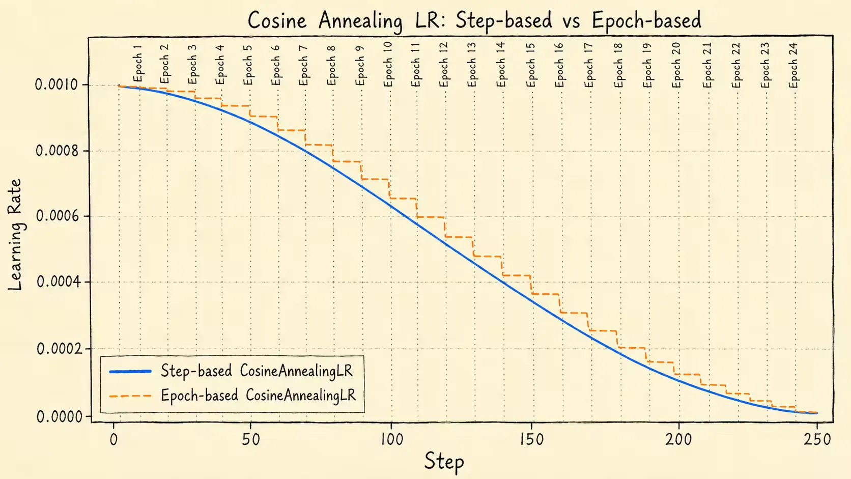
前面介绍优化器时,学习率η \eta η epoch-based \text{epoch-based} epoch-based step-based \text{step-based} step-based
下面介绍几类常见学习率调度器
余弦调度器
由图可知,step-based \text{step-based} step-based step \text{step} step epoch-based \text{epoch-based} epoch-based epoch \text{epoch} epoch epoch \text{epoch} epoch step \text{step} step
通常情况下,1 epoch \text{1 epoch} 1 epoch num batches \text{num batches} num batches step \text{step} step
η t = η m i n + 1 2 ( η m a x − η m i n ) ( 1 + cos ( t T max π ) ) \eta_{t} = \eta_{min} + \frac{1}{2}(\eta_{max} - \eta_{min})\left( 1 + \cos\left( \frac{t}{T_{\text{max}}} \pi\right) \right) η t = η min + 2 1 ( η ma x − η min ) ( 1 + cos ( T max t π ) ) 其中,t t t step \text{step} step epoch \text{epoch} epoch 0 ≤ t ≤ T max 0\leq t\leq T_{\text{max}} 0 ≤ t ≤ T max
线性调度器
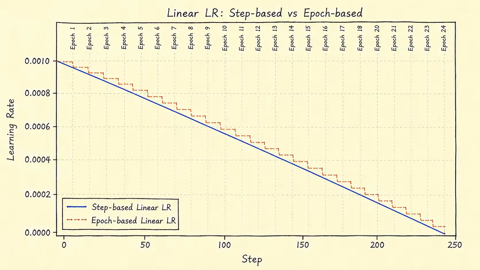
线性调度器按照固定斜率从η max \eta_{\text{max}} η max η min \eta_{\text{min}} η min
η t = η max − t T max ( η max − η min ) \eta_{t} = \eta_{\text{max}} - \frac{t}{T_{\text{max}}}(\eta_{\text{max}} - \eta_{\text{min}}) η t = η max − T max t ( η max − η min ) 其中,t t t step \text{step} step epoch \text{epoch} epoch 0 ≤ t ≤ T max 0\leq t\leq T_{\text{max}} 0 ≤ t ≤ T max
多项式调度器
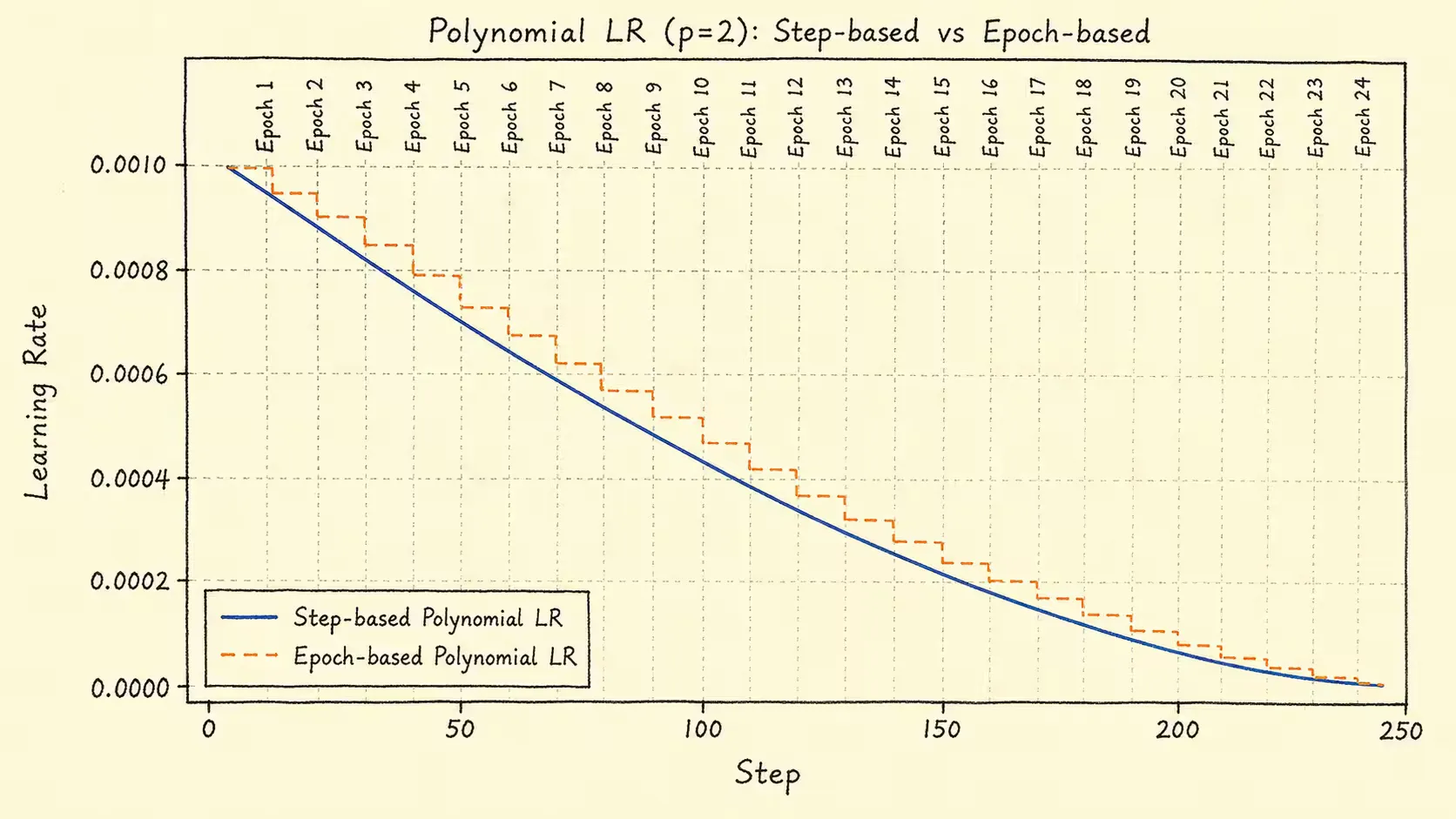
多项式调度器使用幂函数控制学习率衰减曲线,公式为:
η t = η min + ( η max − η min ) ( 1 − t T max ) p \eta_{t} = \eta_{\text{min}} + (\eta_{\text{max}} - \eta_{\text{min}})\left( 1 - \frac{t}{T_{\text{max}}} \right)^p η t = η min + ( η max − η min ) ( 1 − T max t ) p 其中,t t t step \text{step} step epoch \text{epoch} epoch p p p 0 ≤ t ≤ T max 0\leq t\leq T_{\text{max}} 0 ≤ t ≤ T max
预热调度器
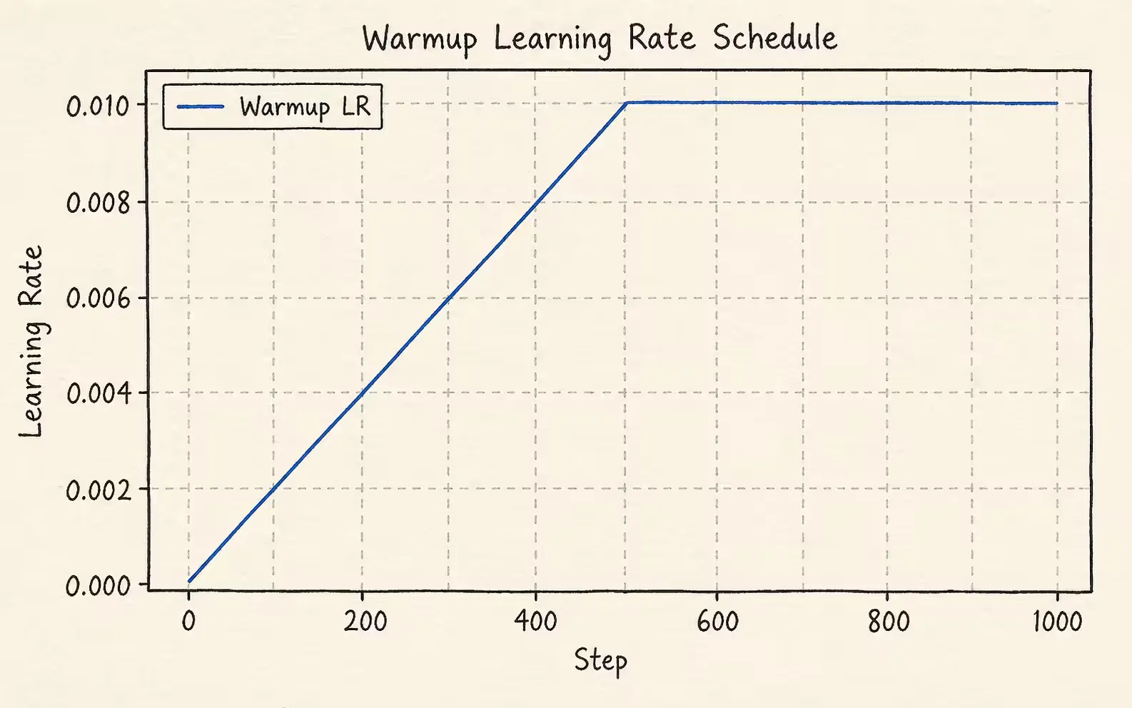
预热调度器通常使用step \text{step} step epoch \text{epoch} epoch warmup \text{warmup} warmup
梯度累积优化
使用单卡GPU训练时,如果批次大小设置过大,很容易出现显存不足。因此,单卡训练通常会使用较小的批次大小
但小批量训练会带来更强的梯度噪声,可能导致损失曲线震荡,甚至影响收敛稳定性。为缓解这一问题,可以使用梯度累积优化
假设小批量大小为b s b_{s} b s B s B_{s} B s B s = n ⋅ b s B_{s}=n\:\cdot b_{s} B s = n ⋅ b s n n n step \text{step} step
在累积期间参数θ t \boldsymbol{\theta}_{t} θ t n n n b s b_{s} b s B s B_{s} B s
g t = 1 n ∑ i = 1 n g t i = 1 n ∑ i = 1 n 1 b s ∇ θ ∑ j = 1 b s L ( x i j , θ t ) = 1 n b s ∑ i = 1 n ∑ j = 1 b s ∇ θ L ( x i j , θ t ) = 1 B s ∇ θ ∑ i = 1 B s L ( x i , θ t ) \begin{align}
\boldsymbol{g}_{t} &= \frac{1}{n}\sum_{i=1}^n\boldsymbol{g}_{t}^i\\
&= \frac{1}{n}\sum_{i=1}^n \frac{1}{b_{s}}\nabla_{\boldsymbol{\theta}}\sum_{j=1}^{b_{s}}\mathcal{L}(\mathbf{x}_{i}^j, \boldsymbol{\theta}_{t}) \\
&= \frac{1}{nb_{s}}\sum_{i=1}^n\sum_{j=1}^{b_{s}}\nabla_{\boldsymbol{\theta}}\mathcal{L}(\mathbf{x}_{i}^j, \boldsymbol{\theta}_{t}) \\
&= \frac{1}{B_{s}}\nabla_{\boldsymbol{\theta}}\sum_{i=1}^{B_{s}}\mathcal{L}(\mathbf{x}^i, \boldsymbol{\theta}_{t})
\end{align} g t = n 1 i = 1 ∑ n g t i = n 1 i = 1 ∑ n b s 1 ∇ θ j = 1 ∑ b s L ( x i j , θ t ) = n b s 1 i = 1 ∑ n j = 1 ∑ b s ∇ θ L ( x i j , θ t ) = B s 1 ∇ θ i = 1 ∑ B s L ( x i , θ t ) 标签平滑
标签平滑是分类任务中的一种正则化技术。它会将原始真实标签,也就是one-hot编码,转换为更柔和的软标签
具体来说,正确类别的概率不再设为1 1 1 1 − ϵ 1-\epsilon 1 − ϵ ϵ \epsilon ϵ K K K
一种常见定义为:
q k = { 1 − ϵ , k = y ϵ K − 1 , k ≠ y q_k =
\begin{cases}
1-\epsilon, & k=y \\
\frac{\epsilon}{K-1}, & k\ne y
\end{cases} q k = { 1 − ϵ , K − 1 ϵ , k = y k = y 模型输出的分类分布为:
p ( y ∣ z ) = s o f t m a x y ( z ) = exp [ z y ] ∑ y ′ = 1 K exp [ z y ′ ] p(y\mid\mathbf{z})=\mathrm{softmax}_{y}(\mathbf{z})=\frac{\exp[z_{y}]}{\sum_{y'=1}^{K}\exp[z_{y'}]} p ( y ∣ z ) = softmax y ( z ) = ∑ y ′ = 1 K exp [ z y ′ ] exp [ z y ] 对正确类别概率取负log \log log
− log p ( y ∣ z ) = − log [ s o f t m a x y ( z ) ] = − log [ exp [ z y ] ∑ y ′ = 1 K exp [ z y ′ ] ] -\log p(y\mid\mathbf{z})=-\log[\mathrm{softmax}_{y}(\mathbf{z})]=-\log\left[\frac{\exp[z_{y}]}{\sum_{y'=1}^{K}\exp[z_{y'}]}\right] − log p ( y ∣ z ) = − log [ softmax y ( z )] = − log [ ∑ y ′ = 1 K exp [ z y ′ ] exp [ z y ] ] − ∇ z log [ s o f t m a x y ( z ) ] = s o f t m a x ( z ) − e y -\nabla_{\mathbf{z}}\log[\mathrm{softmax}_{y}(\mathbf{z})] = \mathrm{softmax}(\mathbf{z}) - \mathbf{e}_{y} − ∇ z log [ softmax y ( z )] = softmax ( z ) − e y 这个梯度说明,普通交叉熵会推动模型输出s o f t m a x ( z ) \mathrm{softmax}(\mathbf{z}) softmax ( z ) e y \mathbf{e}_{y} e y
引入标签平滑后,模型输出分类分布和软标签分布分别为:
p ( y = k ∣ z ) = s o f t m a x k ( z ) = exp [ z k ] ∑ k ′ = 1 K exp [ z k ′ ] p(y=k\mid\mathbf{z})=\mathrm{softmax}_{k}(\mathbf{z})=\frac{\exp[z_{k}]}{\sum_{k'=1}^{K}\exp[z_{k'}]} p ( y = k ∣ z ) = softmax k ( z ) = ∑ k ′ = 1 K exp [ z k ′ ] exp [ z k ] p ( y = k ) = q k p(y=k) = q_{k} p ( y = k ) = q k 两个分布的交叉熵为:
H ( p ( y = k ) , p ( y = k ∣ z ) ) = − ∑ k = 1 K q k log [ exp [ z k ] ∑ k ′ = 1 K exp [ z k ′ ] ] H(p(y=k), p(y=k\mid\mathbf{z})) = -\sum_{k=1}^K q_{k}\log\left[\frac{\exp[z_{k}]}{\sum_{k'=1}^{K}\exp[z_{k'}]}\right] H ( p ( y = k ) , p ( y = k ∣ z )) = − k = 1 ∑ K q k log [ ∑ k ′ = 1 K exp [ z k ′ ] exp [ z k ] ] 最小化该交叉熵等价于最小化两个分布的K L \mathrm{KL} KL
∇ z H ( p ( y = k ) , p ( y = k ∣ z ) ) = s o f t m a x ( z ) − y \nabla_{\mathbf{z}}H(p(y=k), p(y=k\mid\mathbf{z})) = \mathrm{softmax}(\mathbf{z}) - \mathbf{y} ∇ z H ( p ( y = k ) , p ( y = k ∣ z )) = softmax ( z ) − y 因此,标签平滑后的优化目标不再是逼近尖锐的one-hot分布,而是让s o f t m a x ( z ) \mathrm{softmax}(\mathbf{z}) softmax ( z ) y \mathbf{y} y
指数移动平均
前面介绍优化器时,已经多次用到移动平均思想。优化器中的移动平均通常作用于梯度或梯度平方,用来稳定更新方向和更新尺度
模型的指数移动平均(EMA)则作用于权重本身。它会维护一份更平滑的权重副本,常用于提升模型在验证集或测试集上的泛化表现
e m a t + 1 = ρ ⋅ e m a t + ( 1 − ρ ) ⋅ w t \mathbf{ema}_{t+1} = \rho \cdot\mathbf{ema}_{t} + (1 - \rho)\cdot \mathbf{w}_{t} ema t + 1 = ρ ⋅ ema t + ( 1 − ρ ) ⋅ w t 其中,w t \mathbf{w}_{t} w t t t t e m a 0 = w 0 \mathbf{ema}_{0}=\mathbf{w}_{0} ema 0 = w 0
其他训练技巧
除了上面几类方法,训练中还经常使用一些局部技巧。例如,梯度裁剪可以限制梯度范数,缓解梯度爆炸问题:
g ~ t = n m a x max ( ∥ g t ∥ p , n m a x ) g t \tilde{\boldsymbol{g}}_{t}=\frac{\mathrm{n_{max}}}{\max(\lVert \boldsymbol{g}_{t} \rVert_{p}, \mathrm{n_{max}})}\boldsymbol{g}_{t} g ~ t = max (∥ g t ∥ p , n max ) n max g t 早停策略可以在验证集指标不再提升时停止训练,降低过拟合风险。混合精度计算(AMP)则可以减少显存占用,并在合适硬件上提升训练速度
总结
模型训练的优化可以从多个层面展开:优化器决定参数更新方式,调度器控制学习率变化,梯度累积缓解显存限制,标签平滑调整监督信号,EMA则让最终权重更加平稳
这些方法并不是彼此独立的技巧集合,而是共同服务于同一个目标:在有限算力和有限数据下,让训练过程更稳定、收敛更可靠,并尽可能提升模型的泛化能力